Evaluate classification rules in decision-rules
In this tutorial we will evaluate decision rules for regression.
First, we load the boston housing dataset. The column MEDV (median house price in $1000s) is our target variable y, the other ones are the predictors X.
[1]:
import pandas as pd
df = pd.read_csv('resources/boston.csv')
display(df)
X = df.drop(columns=['MEDV'])
y = df['MEDV']
| CRIM | ZN | INDUS | CHAS | NOX | RM | AGE | DIS | RAD | TAX | PTRATIO | B | LSTAT | MEDV | |
|---|---|---|---|---|---|---|---|---|---|---|---|---|---|---|
| 0 | 0.00632 | 18 | 2.31 | 0 | 0.538 | 6.575 | 65.2 | 4.0900 | 1 | 296 | 15 | 396.90 | 4.98 | 24.0 |
| 1 | 0.02731 | 0 | 7.07 | 0 | 0.469 | 6.421 | 78.9 | 4.9671 | 2 | 242 | 17 | 396.90 | 9.14 | 21.6 |
| 2 | 0.02729 | 0 | 7.07 | 0 | 0.469 | 7.185 | 61.1 | 4.9671 | 2 | 242 | 17 | 392.83 | 4.03 | 34.7 |
| 3 | 0.03237 | 0 | 2.18 | 0 | 0.458 | 6.998 | 45.8 | 6.0622 | 3 | 222 | 18 | 394.63 | 2.94 | 33.4 |
| 4 | 0.06905 | 0 | 2.18 | 0 | 0.458 | 7.147 | 54.2 | 6.0622 | 3 | 222 | 18 | 396.90 | 5.33 | 36.2 |
| ... | ... | ... | ... | ... | ... | ... | ... | ... | ... | ... | ... | ... | ... | ... |
| 501 | 0.06263 | 0 | 11.93 | 0 | 0.573 | 6.593 | 69.1 | 2.4786 | 1 | 273 | 21 | 391.99 | 9.67 | 22.4 |
| 502 | 0.04527 | 0 | 11.93 | 0 | 0.573 | 6.120 | 76.7 | 2.2875 | 1 | 273 | 21 | 396.90 | 9.08 | 20.6 |
| 503 | 0.06076 | 0 | 11.93 | 0 | 0.573 | 6.976 | 91.0 | 2.1675 | 1 | 273 | 21 | 396.90 | 5.64 | 23.9 |
| 504 | 0.10959 | 0 | 11.93 | 0 | 0.573 | 6.794 | 89.3 | 2.3889 | 1 | 273 | 21 | 393.45 | 6.48 | 22.0 |
| 505 | 0.04741 | 0 | 11.93 | 0 | 0.573 | 6.030 | 80.8 | 2.5050 | 1 | 273 | 21 | 396.90 | 7.88 | 11.9 |
506 rows × 14 columns
We want to predict the values of y from X using a set of decision rules. The rules are already created, we will load them from a JSON file.
[2]:
import json

from decision_rules import measures
from decision_rules.serialization import JSONSerializer
from decision_rules.regression.ruleset import RegressionRuleSet

# Read the JSON file.
ruleset_path = 'resources/boston_ruleset.json'
with open(ruleset_path) as fp:
    json_ruleset = json.load(fp)

# Create a RegressionRuleSet object from the dict that was stored in JSON.
ruleset: RegressionRuleSet = JSONSerializer.deserialize(json_ruleset, RegressionRuleSet)
ruleset.update(X, y, measure=measures.c2)
# Print the rules in the rule set.
for rule in ruleset.rules:
    print(rule)
IF AGE >= 16.35 AND PTRATIO < 17.50 AND RM >= 7.48 AND LSTAT < 6.25 THEN MEDV = {47.78} [44.45, 51.11] (p=17, n=2, P=23, N=483)
IF RM < 8.35 AND ZN < 92.50 AND CRIM < 0.59 AND CRIM >= 0.02 AND RM >= 7.42 THEN MEDV = {43.01} [38.58, 47.43] (p=13, n=6, P=14, N=492)
IF LSTAT >= 3.15 AND RM < 8.32 AND CRIM >= 0.04 AND INDUS < 18.84 AND AGE >= 24.45 AND RM >= 7.26 THEN MEDV = {36.57} [27.64, 45.49] (p=16, n=5, P=85, N=421)
IF RM < 7.28 AND PTRATIO < 18.50 AND ZN < 92.50 AND CRIM >= 0.01 AND CHAS < 0.50 AND B >= 363.19 AND RM >= 7.08 THEN MEDV = {35.09} [33.44, 36.74] (p=9, n=3, P=16, N=490)
IF AGE < 82.95 AND INDUS >= 1.34 AND LSTAT < 9.10 AND NOX >= 0.40 AND DIS < 9.06 THEN MEDV = {28.86} [21.29, 36.43] (p=110, n=31, P=211, N=295)
IF DIS < 1.89 AND DIS >= 1.50 AND CRIM >= 13.08 AND CRIM < 43.64 AND NOX >= 0.66 THEN MEDV = {9.09} [7.17, 11.02] (p=11, n=2, P=29, N=477)
IF LSTAT >= 20.70 AND LSTAT < 33.01 AND CRIM < 43.64 AND DIS >= 1.37 AND CRIM >= 11.34 AND NOX >= 0.66 THEN MEDV = {9.02} [7.08, 10.96] (p=16, n=3, P=28, N=478)
IF CRIM < 32.15 AND CRIM >= 6.99 AND NOX >= 0.66 THEN MEDV = {12.23} [6.30, 18.16] (p=53, n=2, P=147, N=359)
IF DIS >= 1.18 AND NOX < 0.72 AND DIS < 2.76 AND RM < 7.14 AND NOX >= 0.66 AND CRIM >= 6.60 THEN MEDV = {11.06} [6.95, 15.18] (p=39, n=7, P=94, N=412)
IF RM >= 4.33 AND CRIM >= 6.84 AND CHAS < 0.50 THEN MEDV = {13.06} [7.00, 19.12] (p=70, n=11, P=175, N=331)
IF RM < 7.17 AND TAX >= 222.50 AND AGE >= 28.25 AND LSTAT < 7.96 THEN MEDV = {26.67} [20.21, 33.13] (p=61, n=5, P=225, N=281)
IF RM < 6.44 AND TAX >= 223.50 AND CHAS < 0.50 AND LSTAT < 10.14 AND CRIM < 30.18 THEN MEDV = {23.00} [18.05, 27.95] (p=75, n=4, P=253, N=253)
IF CRIM < 0.57 AND RM >= 6.43 AND LSTAT < 9.92 THEN MEDV = {31.93} [24.31, 39.55] (p=84, n=38, P=116, N=390)
IF CRIM < 7.53 AND LSTAT >= 9.43 AND AGE >= 28.00 AND B >= 363.17 AND RM < 6.95 THEN MEDV = {19.97} [16.57, 23.36] (p=128, n=41, P=211, N=295)
IF B < 396.55 AND CRIM < 6.99 AND CHAS < 0.50 AND B >= 86.04 AND AGE >= 84.50 AND LSTAT >= 14.43 THEN MEDV = {16.22} [12.89, 19.55] (p=49, n=6, P=144, N=362)
IF LSTAT >= 10.54 AND CRIM < 7.25 AND INDUS >= 7.17 AND DIS < 3.97 AND RM < 6.43 AND CRIM >= 0.13 AND INDUS < 20.73 AND RM >= 5.38 AND LSTAT < 14.14 THEN MEDV = {20.65} [18.59, 22.70] (p=23, n=8, P=142, N=364)
IF B >= 6.50 AND B < 368.37 AND CRIM < 7.90 AND RM >= 5.41 AND LSTAT >= 14.40 THEN MEDV = {15.36} [12.41, 18.31] (p=27, n=7, P=109, N=397)
The rule set is loaded and ready for prediction. Let’s generate predictions for the examples in the dataset.
[3]:
y_pred = ruleset.predict(X)
df['MEDV_pred'] = y_pred
display(df)
| CRIM | ZN | INDUS | CHAS | NOX | RM | AGE | DIS | RAD | TAX | PTRATIO | B | LSTAT | MEDV | MEDV_pred | |
|---|---|---|---|---|---|---|---|---|---|---|---|---|---|---|---|
| 0 | 0.00632 | 18 | 2.31 | 0 | 0.538 | 6.575 | 65.2 | 4.0900 | 1 | 296 | 15 | 396.90 | 4.98 | 24.0 | 29.104371 |
| 1 | 0.02731 | 0 | 7.07 | 0 | 0.469 | 6.421 | 78.9 | 4.9671 | 2 | 242 | 17 | 396.90 | 9.14 | 21.6 | 22.998734 |
| 2 | 0.02729 | 0 | 7.07 | 0 | 0.469 | 7.185 | 61.1 | 4.9671 | 2 | 242 | 17 | 392.83 | 4.03 | 34.7 | 32.171973 |
| 3 | 0.03237 | 0 | 2.18 | 0 | 0.458 | 6.998 | 45.8 | 6.0622 | 3 | 222 | 18 | 394.63 | 2.94 | 33.4 | 30.458412 |
| 4 | 0.06905 | 0 | 2.18 | 0 | 0.458 | 7.147 | 54.2 | 6.0622 | 3 | 222 | 18 | 396.90 | 5.33 | 36.2 | 32.171973 |
| ... | ... | ... | ... | ... | ... | ... | ... | ... | ... | ... | ... | ... | ... | ... | ... |
| 501 | 0.06263 | 0 | 11.93 | 0 | 0.573 | 6.593 | 69.1 | 2.4786 | 1 | 273 | 21 | 391.99 | 9.67 | 22.4 | 26.221980 |
| 502 | 0.04527 | 0 | 11.93 | 0 | 0.573 | 6.120 | 76.7 | 2.2875 | 1 | 273 | 21 | 396.90 | 9.08 | 20.6 | 25.626787 |
| 503 | 0.06076 | 0 | 11.93 | 0 | 0.573 | 6.976 | 91.0 | 2.1675 | 1 | 273 | 21 | 396.90 | 5.64 | 23.9 | 29.214162 |
| 504 | 0.10959 | 0 | 11.93 | 0 | 0.573 | 6.794 | 89.3 | 2.3889 | 1 | 273 | 21 | 393.45 | 6.48 | 22.0 | 29.214162 |
| 505 | 0.04741 | 0 | 11.93 | 0 | 0.573 | 6.030 | 80.8 | 2.5050 | 1 | 273 | 21 | 396.90 | 7.88 | 11.9 | 25.982855 |
506 rows × 15 columns
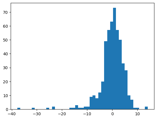
We can calculate the basic regression metrics using calculate_for_regression. The returned value is a dict with keys:
general: general metrics, such as RMSE.histogram: a histogram of errors.
[4]:
from decision_rules.regression.prediction_indicators import calculate_for_regression
import matplotlib.pyplot as plt

print('General metrics')
metrics = calculate_for_regression(y, y_pred)
display(metrics['general'])

print('Histogram of errors')
bins = metrics['histogram']['bin_edges']
counts = metrics['histogram']['histogram']
_ = plt.stairs(counts, bins, fill=True)
General metrics
{'RMSE': 4.90202509087278,
 'MAE': 3.2308461981595062,
 'MAPE': 0.15617752551676722,
 'rRMSE': 0.21755058026782434,
 'rMAE': 0.14338410190400555,
 'maxError': 37.77272727272727,
 'R^2': 0.7153520927414723}
Histogram of errors
The coverage matrix shows which rules cover each of the examples. We can calculate it calling the calculate_coverage_matrix function of the ruleset object. It accepts one argument X which is a DataFrame of examples to check.
The function returns a 2D boolean numpy array. Number of rows is equal to the number of rows (examples) in X and number of columns is the same as the number of rules in the rule set. A True value means that the example is covered by the rule.
[5]:
coverage_matrix = ruleset.calculate_coverage_matrix(X.iloc[:5])
display(coverage_matrix)
print(f'Number of examples: {coverage_matrix.shape[0]}')
print(f'Number of rules: {coverage_matrix.shape[1]}')
array([[False, False, False, False,  True, False, False, False, False,
        False,  True, False,  True, False, False, False, False],
       [False, False, False, False, False, False, False, False, False,
        False, False,  True, False, False, False, False, False],
       [False, False, False,  True,  True, False, False, False, False,
        False, False, False,  True, False, False, False, False],
       [False, False, False, False,  True, False, False, False, False,
        False, False, False,  True, False, False, False, False],
       [False, False, False,  True,  True, False, False, False, False,
        False, False, False,  True, False, False, False, False]])
Number of examples: 5
Number of rules: 17
The calculate_rules_metrics function of a ruleset object computes metrics describing each of the rules in the rule set. The explanations of the metrics can be found in the documentation of ruleminer.
[ ]:
metrics = ruleset.calculate_rules_metrics(X, y)
for rule_id, metrics in metrics.items():
    print('Rule', rule_id)
    print(metrics)
Rule fc70c54b-02f9-4cd5-81d0-7f73d85dc367
{'p': 17, 'n': 2, 'P': 23, 'N': 483, 'p_unique': 17, 'n_unique': 17, 'support': 19, 'conditions_count': 4, 'y_covered_avg': 47.77894736842106, 'y_covered_median': 50.0, 'y_covered_min': 37.6, 'y_covered_max': 50.0, 'mae': 25.395548158934893, 'rmse': 26.8660974796374, 'mape': 1.5125990035583592, 'p-value': 4.231965993998835e-06}
Rule 1634ea74-f2aa-400b-8ba4-1b658578b00a
{'p': 13, 'n': 6, 'P': 14, 'N': 492, 'p_unique': 13, 'n_unique': 13, 'support': 19, 'conditions_count': 5, 'y_covered_avg': 43.00526315789473, 'y_covered_median': 43.5, 'y_covered_min': 33.4, 'y_covered_max': 50.0, 'mae': 21.032764718119402, 'rmse': 22.439720251538724, 'mape': 1.2702153772414488, 'p-value': 0.00032332389088428164}
Rule cdc83a4b-d169-4372-a508-af418d02b556
{'p': 16, 'n': 5, 'P': 85, 'N': 421, 'p_unique': 16, 'n_unique': 16, 'support': 21, 'conditions_count': 6, 'y_covered_avg': 36.56666666666666, 'y_covered_median': 35.2, 'y_covered_min': 15.0, 'y_covered_max': 50.0, 'mae': 15.40527009222661, 'rmse': 16.774051158576192, 'mape': 0.9493332806979319, 'p-value': 0.46645377271528804}
Rule 6fb80d0a-b7ae-4325-8c5e-76226b8d2a03
{'p': 9, 'n': 3, 'P': 16, 'N': 490, 'p_unique': 9, 'n_unique': 9, 'support': 12, 'conditions_count': 7, 'y_covered_avg': 35.091666666666676, 'y_covered_median': 35.15, 'y_covered_min': 31.6, 'y_covered_max': 37.9, 'mae': 14.181785243741773, 'rmse': 15.560993839083396, 'mape': 0.8775897305716386, 'p-value': 2.1589703599932363e-07}
Rule a6d5f154-e5d8-42a7-a7fb-7999ee8edfdc
{'p': 110, 'n': 31, 'P': 211, 'N': 295, 'p_unique': 110, 'n_unique': 110, 'support': 141, 'conditions_count': 5, 'y_covered_avg': 28.858156028368793, 'y_covered_median': 26.6, 'y_covered_min': 11.9, 'y_covered_max': 50.0, 'mae': 9.648011100832562, 'rmse': 11.154801882477512, 'mape': 0.5935712142448168, 'p-value': 0.00125917486075591}
Rule 7666c01f-c21d-409b-9162-c1450927bfee
{'p': 11, 'n': 2, 'P': 29, 'N': 477, 'p_unique': 11, 'n_unique': 11, 'support': 13, 'conditions_count': 5, 'y_covered_avg': 9.092307692307696, 'y_covered_median': 8.5, 'y_covered_min': 5.6, 'y_covered_max': 12.7, 'mae': 13.573852234721796, 'rmse': 16.280864830458583, 'mape': 0.5432146614616068, 'p-value': 3.648142869045188e-07}
Rule 13f4ff45-93e7-4bd3-b6bd-8658d2f00063
{'p': 16, 'n': 3, 'P': 28, 'N': 478, 'p_unique': 16, 'n_unique': 16, 'support': 19, 'conditions_count': 6, 'y_covered_avg': 9.021052631578947, 'y_covered_median': 8.8, 'y_covered_min': 5.0, 'y_covered_max': 13.1, 'mae': 13.639192843769504, 'rmse': 16.339738186513586, 'mape': 0.546143930494049, 'p-value': 4.972293644367493e-10}
Rule 66b5f17f-130f-4758-bba2-d5773a8ae8d2
{'p': 53, 'n': 2, 'P': 147, 'N': 359, 'p_unique': 53, 'n_unique': 53, 'support': 55, 'conditions_count': 3, 'y_covered_avg': 12.227272727272727, 'y_covered_median': 11.7, 'y_covered_min': 5.6, 'y_covered_max': 50.0, 'mae': 10.821451670858785, 'rmse': 13.806649806224579, 'mape': 0.4261063230868248, 'p-value': 4.539164119741508e-05}
Rule 2ef97491-a4fb-44ec-9f4b-5637da1fd9d5
{'p': 39, 'n': 7, 'P': 94, 'N': 412, 'p_unique': 39, 'n_unique': 39, 'support': 46, 'conditions_count': 6, 'y_covered_avg': 11.06304347826087, 'y_covered_median': 10.7, 'y_covered_min': 5.0, 'y_covered_max': 27.9, 'mae': 11.806547516755456, 'rmse': 14.696088455647036, 'mape': 0.46617491141164896, 'p-value': 1.2859048511740222e-09}
Rule 3cffdf44-dc64-4044-b430-ec95e153c4ad
{'p': 70, 'n': 11, 'P': 175, 'N': 331, 'p_unique': 70, 'n_unique': 70, 'support': 81, 'conditions_count': 3, 'y_covered_avg': 13.058024691358028, 'y_covered_median': 12.3, 'y_covered_min': 5.0, 'y_covered_max': 50.0, 'mae': 10.150968623432389, 'rmse': 13.198145443376216, 'mape': 0.4001944889170244, 'p-value': 2.310205784360766e-06}
Rule a974919d-9fbc-49f7-a34a-a23a024ac082
{'p': 61, 'n': 5, 'P': 225, 'N': 281, 'p_unique': 61, 'n_unique': 61, 'support': 66, 'conditions_count': 4, 'y_covered_avg': 26.668181818181818, 'y_covered_median': 24.65, 'y_covered_min': 11.9, 'y_covered_max': 50.0, 'mae': 8.369080129356808, 'rmse': 10.07575737268071, 'mape': 0.5042875491291532, 'p-value': 0.00019747617416798985}
Rule 46605476-d4c6-42cc-8893-9ac43588fe71
{'p': 75, 'n': 4, 'P': 253, 'N': 253, 'p_unique': 75, 'n_unique': 75, 'support': 79, 'conditions_count': 5, 'y_covered_avg': 22.998734177215184, 'y_covered_median': 22.6, 'y_covered_min': 11.9, 'y_covered_max': 50.0, 'mae': 6.743183068994845, 'rmse': 9.199817656913865, 'mape': 0.3749461786251191, 'p-value': 1.0236828474464975e-10}
Rule c5de0cc6-0031-490b-b622-4ea4c43e4690
{'p': 84, 'n': 38, 'P': 116, 'N': 390, 'p_unique': 84, 'n_unique': 84, 'support': 122, 'conditions_count': 3, 'y_covered_avg': 31.9344262295082, 'y_covered_median': 30.950000000000003, 'y_covered_min': 16.5, 'y_covered_max': 50.0, 'mae': 11.740452277586991, 'rmse': 13.145722232031703, 'mape': 0.7291748055269496, 'p-value': 0.0033602885206500148}
Rule dd0ebdad-a5c9-468a-a20a-fb89653b8706
{'p': 128, 'n': 41, 'P': 211, 'N': 295, 'p_unique': 128, 'n_unique': 128, 'support': 169, 'conditions_count': 5, 'y_covered_avg': 19.96568047337278, 'y_covered_median': 19.9, 'y_covered_min': 11.8, 'y_covered_max': 36.2, 'mae': 6.62361952428842, 'rmse': 9.539899962247627, 'mape': 0.3215163752153801, 'p-value': 3.3630561612817378e-43}
Rule 44f26c78-8a18-491b-b123-5062719056d8
{'p': 49, 'n': 6, 'P': 144, 'N': 362, 'p_unique': 49, 'n_unique': 49, 'support': 55, 'conditions_count': 6, 'y_covered_avg': 16.220000000000002, 'y_covered_median': 16.0, 'y_covered_min': 7.0, 'y_covered_max': 30.7, 'mae': 8.08403162055336, 'rmse': 11.147693924839217, 'mape': 0.3367071061321477, 'p-value': 1.9183487774190778e-15}
Rule 2bb7b89b-b885-4944-b1b8-1648064d4f13
{'p': 23, 'n': 8, 'P': 142, 'N': 364, 'p_unique': 23, 'n_unique': 23, 'support': 31, 'conditions_count': 9, 'y_covered_avg': 20.64516129032258, 'y_covered_median': 20.6, 'y_covered_min': 16.1, 'y_covered_max': 24.5, 'mae': 6.547303327808237, 'rmse': 9.3799125758053, 'mape': 0.3286167130929514, 'p-value': 5.067990050751164e-15}
Rule 2d879e71-b475-4cc4-9a5f-f525a2f927d9
{'p': 27, 'n': 7, 'P': 109, 'N': 397, 'p_unique': 27, 'n_unique': 27, 'support': 34, 'conditions_count': 5, 'y_covered_avg': 15.358823529411763, 'y_covered_median': 15.05, 'y_covered_min': 7.0, 'y_covered_max': 23.7, 'mae': 8.5747733085329, 'rmse': 11.656997267512827, 'mape': 0.3491076881259912, 'p-value': 1.4991455332547193e-11}
The calculate_ruleset_stats function returns some general statistics regarding the rules present in the rule set.
[7]:
general_stats = ruleset.calculate_ruleset_stats()
print(general_stats)
{'rules_count': 17, 'avg_conditions_count': 5.12, 'avg_precision': 0.82, 'avg_coverage': 0.45, 'total_conditions_count': 87}
We can use calculate_condition_importances and calculate_attribute_importances to find the importances of conditions in the rules and consequently the importances of attributes in the data set.
[ ]:
condition_importances = ruleset.calculate_condition_importances(X, y, measure=measures.c2)
display(condition_importances)
[{'condition': 'NOX >= 0.66',
  'attributes': ['NOX'],
  'importance': 0.41219564492890814},
 {'condition': 'CRIM >= 6.84',
  'attributes': ['CRIM'],
  'importance': 0.3463070344654806},
 {'condition': 'RM >= 7.48',
  'attributes': ['RM'],
  'importance': 0.28703662615958525},
 {'condition': 'CRIM >= 6.99',
  'attributes': ['CRIM'],
  'importance': 0.2581918553894471},
 {'condition': 'RM >= 7.42',
  'attributes': ['RM'],
  'importance': 0.21428470226221466},
 {'condition': 'LSTAT < 7.96',
  'attributes': ['LSTAT'],
  'importance': 0.1841743175107864},
 {'condition': 'RM >= 7.26',
  'attributes': ['RM'],
  'importance': 0.17189228602638446},
 {'condition': 'LSTAT < 9.92',
  'attributes': ['LSTAT'],
  'importance': 0.1597209591117324},
 {'condition': 'LSTAT < 10.14',
  'attributes': ['LSTAT'],
  'importance': 0.13977988686201942},
 {'condition': 'LSTAT >= 14.43',
  'attributes': ['LSTAT'],
  'importance': 0.13474623065608687},
 {'condition': 'CRIM < 0.57',
  'attributes': ['CRIM'],
  'importance': 0.13236275435336914},
 {'condition': 'CRIM >= 13.08',
  'attributes': ['CRIM'],
  'importance': 0.12967575688395577},
 {'condition': 'LSTAT >= 14.40',
  'attributes': ['LSTAT'],
  'importance': 0.12762735615087725},
 {'condition': 'RM >= 7.08',
  'attributes': ['RM'],
  'importance': 0.11911032403269536},
 {'condition': 'LSTAT < 9.10',
  'attributes': ['LSTAT'],
  'importance': 0.11608645865167616},
 {'condition': 'CRIM >= 11.34',
  'attributes': ['CRIM'],
  'importance': 0.10957886720572627},
 {'condition': 'RM < 6.44',
  'attributes': ['RM'],
  'importance': 0.10721755983765796},
 {'condition': 'CRIM >= 6.60',
  'attributes': ['CRIM'],
  'importance': 0.107037596978978},
 {'condition': 'LSTAT < 6.25',
  'attributes': ['LSTAT'],
  'importance': 0.09987681138116272},
 {'condition': 'CRIM < 0.59',
  'attributes': ['CRIM'],
  'importance': 0.0972942505053715},
 {'condition': 'NOX >= 0.66',
  'attributes': ['NOX'],
  'importance': 0.09443159057752622},
 {'condition': 'RM < 7.17',
  'attributes': ['RM'],
  'importance': 0.08864968911934279},
 {'condition': 'LSTAT >= 9.43',
  'attributes': ['LSTAT'],
  'importance': 0.08830877842262368},
 {'condition': 'LSTAT >= 20.70',
  'attributes': ['LSTAT'],
  'importance': 0.08364177051884032},
 {'condition': 'PTRATIO < 17.50',
  'attributes': ['PTRATIO'],
  'importance': 0.0812812354219555},
 {'condition': 'AGE < 82.95',
  'attributes': ['AGE'],
  'importance': 0.07470814962300586},
 {'condition': 'RM >= 6.43',
  'attributes': ['RM'],
  'importance': 0.07395685376026782},
 {'condition': 'CRIM < 7.53',
  'attributes': ['CRIM'],
  'importance': 0.06852878406567027},
 {'condition': 'LSTAT < 14.14',
  'attributes': ['LSTAT'],
  'importance': 0.06500338170219208},
 {'condition': 'CRIM < 7.90',
  'attributes': ['CRIM'],
  'importance': 0.06484694679647318},
 {'condition': 'RM < 6.95',
  'attributes': ['RM'],
  'importance': 0.06142012277300351},
 {'condition': 'CRIM < 6.99',
  'attributes': ['CRIM'],
  'importance': 0.06072283131891407},
 {'condition': 'DIS < 1.89',
  'attributes': ['DIS'],
  'importance': 0.05913420105949188},
 {'condition': 'CHAS < 0.50',
  'attributes': ['CHAS'],
  'importance': 0.05575023428251599},
 {'condition': 'B < 368.37',
  'attributes': ['B'],
  'importance': 0.052711629950983545},
 {'condition': 'LSTAT >= 10.54',
  'attributes': ['LSTAT'],
  'importance': 0.052079922998162276},
 {'condition': 'RM < 6.43',
  'attributes': ['RM'],
  'importance': 0.048826126018804365},
 {'condition': 'AGE >= 84.50',
  'attributes': ['AGE'],
  'importance': 0.04776356065683929},
 {'condition': 'PTRATIO < 18.50',
  'attributes': ['PTRATIO'],
  'importance': 0.046696713324452715},
 {'condition': 'DIS >= 1.50',
  'attributes': ['DIS'],
  'importance': 0.043589660805792366},
 {'condition': 'B >= 363.17',
  'attributes': ['B'],
  'importance': 0.0433463463241028},
 {'condition': 'ZN < 92.50',
  'attributes': ['ZN'],
  'importance': 0.04309189275034518},
 {'condition': 'INDUS >= 7.17',
  'attributes': ['INDUS'],
  'importance': 0.04185396665287753},
 {'condition': 'CRIM < 43.64',
  'attributes': ['CRIM'],
  'importance': 0.04018867408245981},
 {'condition': 'RM < 7.28',
  'attributes': ['RM'],
  'importance': 0.03903537520801033},
 {'condition': 'RM < 7.14',
  'attributes': ['RM'],
  'importance': 0.038817813173326096},
 {'condition': 'TAX >= 222.50',
  'attributes': ['TAX'],
  'importance': 0.03358080804623055},
 {'condition': 'CRIM < 7.25',
  'attributes': ['CRIM'],
  'importance': 0.029954141206563537},
 {'condition': 'B >= 363.19',
  'attributes': ['B'],
  'importance': 0.029321745968898253},
 {'condition': 'RM < 8.35',
  'attributes': ['RM'],
  'importance': 0.026316696161776582},
 {'condition': 'CRIM < 32.15',
  'attributes': ['CRIM'],
  'importance': 0.02330906239533667},
 {'condition': 'RM < 8.32',
  'attributes': ['RM'],
  'importance': 0.018934742866803526},
 {'condition': 'RM >= 5.41',
  'attributes': ['RM'],
  'importance': 0.018498186505621655},
 {'condition': 'CRIM >= 0.02',
  'attributes': ['CRIM'],
  'importance': 0.017740808626785134},
 {'condition': 'B >= 86.04',
  'attributes': ['B'],
  'importance': 0.01698260625974729},
 {'condition': 'TAX >= 223.50',
  'attributes': ['TAX'],
  'importance': 0.015646623545917445},
 {'condition': 'DIS >= 1.37',
  'attributes': ['DIS'],
  'importance': 0.014608935287077046},
 {'condition': 'NOX < 0.72',
  'attributes': ['NOX'],
  'importance': 0.014313462697020378},
 {'condition': 'CRIM >= 0.04',
  'attributes': ['CRIM'],
  'importance': 0.01426262284060611},
 {'condition': 'LSTAT >= 3.15',
  'attributes': ['LSTAT'],
  'importance': 0.013348883895085673},
 {'condition': 'CRIM >= 0.01',
  'attributes': ['CRIM'],
  'importance': 0.01306363096456618},
 {'condition': 'AGE >= 28.25',
  'attributes': ['AGE'],
  'importance': 0.011369879785042732},
 {'condition': 'RM >= 5.38',
  'attributes': ['RM'],
  'importance': 0.011358876636887215},
 {'condition': 'DIS >= 1.18',
  'attributes': ['DIS'],
  'importance': 0.0110300559444215},
 {'condition': 'CRIM < 30.18',
  'attributes': ['CRIM'],
  'importance': 0.010494744135007401},
 {'condition': 'AGE >= 16.35',
  'attributes': ['AGE'],
  'importance': 0.009804987963755939},
 {'condition': 'CRIM >= 0.13',
  'attributes': ['CRIM'],
  'importance': 0.00925020629003368},
 {'condition': 'DIS < 2.76',
  'attributes': ['DIS'],
  'importance': 0.009243016697363543},
 {'condition': 'B < 396.55',
  'attributes': ['B'],
  'importance': 0.008241849524085656},
 {'condition': 'AGE >= 28.00',
  'attributes': ['AGE'],
  'importance': 0.007296220587578672},
 {'condition': 'RM >= 4.33',
  'attributes': ['RM'],
  'importance': 0.005964485712736271},
 {'condition': 'INDUS >= 1.34',
  'attributes': ['INDUS'],
  'importance': 0.0035914514368505924},
 {'condition': 'LSTAT < 33.01',
  'attributes': ['LSTAT'],
  'importance': 0.003345159046207844},
 {'condition': 'DIS < 9.06',
  'attributes': ['DIS'],
  'importance': 0.003239267344266099},
 {'condition': 'B >= 6.50',
  'attributes': ['B'],
  'importance': 0.003128072049983466},
 {'condition': 'NOX >= 0.40',
  'attributes': ['NOX'],
  'importance': 0.0006305615911450331},
 {'condition': 'INDUS < 20.73',
  'attributes': ['INDUS'],
  'importance': 0.00029380923899731247},
 {'condition': 'AGE >= 24.45',
  'attributes': ['AGE'],
  'importance': -0.0004797895116285027},
 {'condition': 'INDUS < 18.84',
  'attributes': ['INDUS'],
  'importance': -0.0008170150896906769},
 {'condition': 'DIS < 3.97',
  'attributes': ['DIS'],
  'importance': -0.0059103572995956415}]
[9]:
attribute_importances = ruleset.calculate_attribute_importances(condition_importances)
display(attribute_importances)
{'CRIM': 1.5328105685047448,
 'RM': 1.3313204662551184,
 'LSTAT': 1.2677399169074535,
 'NOX': 0.5215712597945998,
 'B': 0.15373225007780103,
 'AGE': 0.150463009104594,
 'DIS': 0.13493477983881683,
 'PTRATIO': 0.12797794874640822,
 'CHAS': 0.05575023428251599,
 'TAX': 0.049227431592148,
 'INDUS': 0.04492221223903476,
 'ZN': 0.04309189275034518}